Rock Mackie 1,2, PhD

John Hayes 1, PhD

1: Asto CT Inc, Middleton, WI USA

2: Medical Physics, University of Wisconsin-Madison, Madison, WI USA

INTRODUCTION

The accessibility of computed tomography (CT) for veterinary indications is increasing, with particular interest in scanning the legs, head, and neck of horses. Equine veterinarians who are considering investing in CT equipment for their practice are faced with a complex choice as they try to identify the technology solution that will most improve their practice. Image quality is one of the key considerations since it will inform the ability of the equine veterinarian to identify pathology and make diagnoses that are not possible using radiography or other standard measurements. This review describes the relative merits of two common methods for acquiring CT imaging: fan-beam and cone-beam imaging.

CT BASICS

Fan-beam and cone-beam scanners differ technically in the manner in which they scan around the subject and with their image sensor characteristics. The original CT scanners were fan-beam and the detector technologies have evolved for 50 years to optimize the speed of acquisition, detector size, detector efficiency and the capacity to accurately represent the measured attenuation. Cone-beam CT detectors evolved in the past 20 years from electronic planar “flat panel” detectors that were developed to directly produce conventional planar x-ray images in place of film radiographs.

The detectors work by stopping the x-rays in light-emitting scintillation layers that convert the x-ray energy into light which is detected in sensors and converted to a digital signal by an analog-to-digital (A2D) convertor and finally stored in electronic memory not unlike those in a modern electronic camera. The electronic data is used by a computer to obtain a representation of the 3D anatomy of a region of the subject in a process called “image reconstruction”.

A fundamental assumption in reconstruction is that the attenuation of x-rays traveling through the subject received by the detector are accurate and that the subject is still. The reconstruction produces, for each volume element (“voxel”) of the representation, numerical values called Hounsfield Numbers (HU) named after the co-inventor of the CT scanner, Godfrey Hounsfield. HU is a quantity proportional to the x-ray attenuation of a voxel as compared to the attenuation had the voxel been water and depends on the energy in kilovolts (kV) of the x-ray beam. Mathematically, HU (kV) is given by:

An HU value of -1000 is vacuum (i.e., no attenuation at all) and 0 HU is water. Dense bone or metal is highly attenuating and there is no upper range limit but can have values significantly higher than 1000 HU. Most soft tissue have values close to that of water.

The 3D numerical representation is typically presented to the clinician as a 2D gray-scale picture called a “slice” representing a thin cross section through the anatomy (Figure 1). The color map of the image mimics standard photographic film with black being low attenuation and white being high attenuation.

Figure 1: A 2D “slice” in the axial plane of a CT image. The lungs—mostly air—are black because they have very low attenuation, while the bones, which are very highly attenuating, are white. (Not captured with the Equina)

TYPES OF SCANNERS

Fan-beam CT scanners use a curved detector surface and rotate around the subject multiple times, acquiring data in the full 360° range. Cone-beam CT scanners use a flat detector surface, and only rotate around the patient a single time on an arc limited typically less than 240°.

Fan-beam CT has a limited number of rows—16 to as high as 256—with about 1200 detector sensors per row. The subject or the scanner is translated along the row direction to image the patient. Today, most fan-beam CT scanners are helical in that the rotation of the scanner and the translation of the subject or scanner are simultaneous, forming a helical path around the subject. Cone-beam CT detectors on the other have a large matrix of sensors up to 2048 columns × 1536 rows. Helical scanning (translation) isn’t done in cone-beam CT because the larger detector size typically captures enough information along the row dimension.

The number of image sensors in a fan-beam CT is much smaller than in cone-beam CT, but the data acquisition rate is orders of magnitude faster. Correspondingly, the speed of acquisition requires scintillators which are very efficient, emit light promptly and have low afterglow characteristics. A commonly used scintillation material is gadolinium oxysulfide (GOS) which has a density of 7.4 g/cm3.

Figure 2: Illustration of the geometry and typical scanner setup for cone-beam and fan-beam CT.

In cone-beam CT, to be able to approach the fine detail of photographic film, the resolution of the detector elements is much finer than needed for CT. However, when used for CT, the detector elements (“pixels") are binned or averaged together (4 x 4 is typical for CT resulting in an effective pixel that measures 0.5 mm x 0.5 mm) to reduce the inherent noise in small area sensors. There is a large area that needs to be coated in flat panel detectors and they typically use less efficient and less costly materials than GOS, such as CsI, which has a density of 4.5 g/cm3. The lower density allows x-rays to go right through without being detected and so some wasted signal leads to a reduced dose efficiency for cone-beam CT as compared to fan-beam CT.

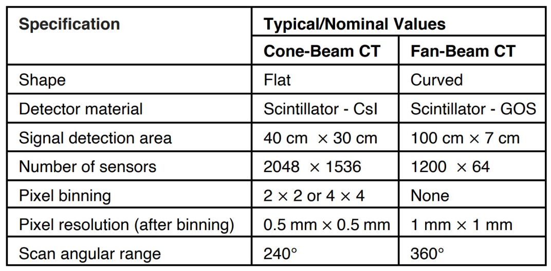
Table 1: Summary of the nominal difference between cone-beam and fan-beam CT systems.

NOISE

Noise in CT detectors can be easily seen as a random “salt and pepper” pattern in the image akin to an old TV set not tuned to a station. The magnitude of the noise however must be compared to the magnitude of the true signal, and this is often expressed by signal-to-noise ratio (SNR is also what matters in a crowded restaurant when you want to carry out a conversation). The higher the SNR, the easier it is to identify anatomy that differs only slightly in density. Another measure of noise is the standard deviation (or error) of HU for a material, with water typically the reference material (as soft tissue has a HU close to water.) Standard deviation of HU for water is measured by imaging a water filled phantom and determining the histogram of voxel values. The mean should be close to zero, and the lower the standard deviation the lower the noise.

For cone-beam CT, binning together smaller pixels rather than having one equivalent larger pixel results in a reduced area that is sensitive to light because an insensitive gap is required between the small pixels. A good analogy is a coin toss game where coins are tossed into separated containers. If the coin hits a rim, it can bounce off and not get collected into any container. A single container catches more coins than a set of smaller containers. The ratio of collected area to total area is called the fill factor and flat-panels used for CT typically have a fill factor around 65% as compared to the detectors in a fan-beam CT of 90%. The reduced signal size from small detector elements and the slow acquisition speed in cone beam detectors (causing accumulated signal being held longer before readout) decrease the signal-to-noise of cone-beam data significantly compared to a fan-beam.

The higher noise inherent in the signals from a cone-beam CT means that the A2D convertors need not digitize with as many possible values as routinely used in processing the signal for a fan beam CT. The “bit depth” of a cone-beam CT is typically 16 bits which means that a signal can be digitized to integer values between 0 and 216-1 or 65,536 possible values. By contrast the bit depth of an A2D of a fan-beam CT is typically 24 bits or 16,777,216 possible values. Although more expensive, the higher bit depth used in fan-beam detector systems allows a larger range of attenuation to be inferred. This also means when one increases radiation dose to boost signal for extremely high attenuating material like metals or other highly dense objects, it is easier to avoid detector saturation for the other paths with very low or no attenuation. It also prevents any further noise than that which results from the fundamental detector quantum noise inherent to x-rays being discrete particles (called photons). Ideally, the noise in a CT image is limited by quantum interactions, not in the error resulting from digitization. When this is so, the only way to reduce noise is to increase dose. Unfortunately, the noise level is inversely proportional to the square root of the dose to the subject, e.g., to halve the noise level, one must quadruple the dose.

RESOLUTION

In CT, as compared to planar radiography, there is a trade-off made to sacrifice lower resolution for improved contrast. A planar radiograph has very fine resolution for high contrast objects such as lung or bone but in a planar radiograph it is impossible to see low contrast objects such as the difference between muscle and fat. The ability to see low contrast is measured by placing known plastic materials in a water phantom and determining if they can be visualized. At the center of a CT reconstruction, which is coincident with the axis of rotation, the resolution and noise of the voxels is dominated by the resolution and the noise of only a few detectors because the center voxels are only reconstructed from information from the central detectors. However, farther away from the axis of rotation the fundamental resolution is dominated by the resolution of the angular sampling and therefore fine detectors do contribute to resolution. In CT, noise is averaged over many detector samples contributing to the voxel values. Depending on the lateral field of view, it takes many hundreds to a few thousand angular views to create adequate data for reconstruction of larger lateral field of views such that small differences in contrast in soft tissue can be easily differentiated.

The modulation transfer function (MTF) is a measure of resolution. The higher the modulation transfer the finer the resolution for high contrast objects. The binned pixels of a cone-beam CT are usually finer than that of a fan-beam CT (typically 1 mm x 1 mm) and so can have greater MTF, however, the MTF also depends on the spot size of the x-ray tube which is typically also on the order of 1 mm in diameter and so there is only a small gain in MTF with pixel sizes less than 1 mm x 1mm.

ARTIFACTS: SCATTER

Cone-beam CT is also more prone to artifacts. The size of an instantaneous field of view in cone-beam CT at the flat detector plane is about 40 cm x 40 cm compared to a fan-beam CT of 5 cm x 60 cm at the curved detector plane which means that there is much more scatter at the flat panel than at the fan-beam detectors. Additionally, there is generally more scatter detected than direct signal for a flat panel detector and there is also more scatter at the center of the image than at the edge. Scatter to a detector is mistaken for signal which is interpreted as less attenuation. If uncorrected, these factors lead to HU inaccuracy and non-uniformity of the image. Under-correcting the scatter signal leads to “cupping” artifacts and over-correcting leads to “capping” artifacts. Non-uniformity is determined by measuring the uniformity of a water phantom. The uniformity index often expressed as a percent, and is the difference between the HU at the center of a water phantom and HU at the periphery normalized to the HU at the center (lower is better). Because there is much less scatter in a fan-beam CT, its uniformity index is smaller than cone-beam CT.

The radiation from a large instantaneous field of view of a cone-beam CT scanner is difficult to shield. In veterinary medicine, the dose to the subject is important but the dose to the handler is even more important. Scattered radiation produced by the horse scatters outside to expose the handler as well. Dose efficiency is therefore very important. Having less scatter arrive at the handler, not wasting photons with poor fill factors in the detector sensors, and having good intrinsic contrast detectability so that the x-ray current (mA) does not have to be increased to see the anatomy are all factors that are superior in fan-beam CT over cone-beam CT.

ARTIFACTS: MOTION

The response to movement of the subject on a cone-beam CT is much worse than that of a fan-beam CT. The reconstruction algorithm is predicated on a motionless subject. Any movement within the full acquisition time of the cone-beam CT means that an artifact will be generated. Typical acquisition times in cone-beam CT can be many seconds to a minute because the sample rate of the flat panel is about 40 per second and good angular resolution on the order of a thousand samples are required for larger lateral fields of view. Gross movements are actually a smaller problem than subtle movements as they can be easily detected and the scan can be repeated. However, subtle artifacts can sometimes be mistaken for diseased pathology. Motion artifacts are less of an issue in fan-beam CT as the speed of acquisition for a slice is a fraction of a second or more than an order of magnitude faster per revolution than for a cone-beam CT. In a fan-beam CT scan of a horse limb when the animal is swaying gently there may be small lateral discontinuities between slices but the anatomy of a slice is well preserved

FIELD OF VIEW

At the present time, there are no cone-beam CT scanners that can scan helically. This is not a practical limitation for some applications if the panels are large enough to acquire a relatively large volume in one rotation. Imaging a whole-body of a human or the limb of a tall horse with a cone-beam CT would require stitching together separate CT image sets. By contrast, a fan-beam CT scanner is inherently designed to scan through just enough rotations to see the pathology and can scan short longitudinal fields of view irradiating only the part of the subject necessary. Fan-beam CT scanners can also scan long fields of view conveniently in one image set.

SUMMARY

Fan-beam and cone-beam scanners both have applications in human medicine with fan-beam systems excelling in diagnostic imaging and cone-beam systems being favored in applications where the positioning of the subject is critical but detailed diagnostic images are not.

In the equine space, fan-beam systems offer several key advantages. Fan-beam systems offer faster scan times which make its images less susceptible to motion artifacts due to swaying or other subtle movements of the equine patient. Fan-beam images also have higher image quality, enabling them to be used to identify subtle pathological changes in the limbs of horses, and important advantage over both traditional radiography and cone-beam CT scanning. Veterinarians considering introducing CT into their equine practice should consider the superior image quality of fan-beam systems when selecting their instrument of choice.

Table 2: Image quality metric comparison of cone-beam and fan-beam CT scanners adapted from Lechuga and Weidlich (Lechuga L, Weidlich G A., September 12, 2016, Cone Beam CT vs. Fan Beam CT: A Comparison of Image Quality and Dose Delivered Between Two Differing CT)

Download Whitepaper

Whitepaper: Fan Beam CT versus Cone Beam CT for Veterinary Medicine